research

Two examples of our activities concerning the combination of models and observations and of testing climate models.

Adjoint method of data assimilation: Combining full-complexity ocean general circulation models with observations, for calculating un-observable quantities and for initiating climate predictions.
Using "transfer functions" to quantitatively test individual physical processes in ocean and climate models. This helps identify systematic and compensating model errors, which may lead to a seemingly satisfactory simulation of present climate, while deteriorating climate prediction skill when model errors stop compensating in a changing climate

Data assimilation: combining ocean models and data:

There are many available observations of the oceanic circulation from research ships, satellites, and moored instruments. However, very often quantities of interest for climate purposes cannot be measured directly. For example, we know quite well the temperature field of the ocean and function of season, geographical location and depth. But there are no direct data of the amount of heat carried by ocean currents from the equator to the poles, which is an important climate unknown. Ocean models may be used to bridge between the available data and desired information. We have been developing a sophisticated method for the assimilation of ocean data into models and for the extraction of the needed climate information. The method is known as the "adjoint method" and is based on "optimal control" theory. The method requires a model that is based on the adjoint equations of the ocean model to which data is assimilated... [1, 2, 3]

In order to predict climate phenomena such as El Nino, one needs to initialize a model of the coupled Pacific ocean and atmosphere with the available data and then run it in a prediction mode. The adjoint method is again useful for this initialization, and in this context is often referred to as "4d variational data assimilation". [1]

Adjoint models can also be used for sensitivity and generalized stability studies, and some relevant results are shown in the figure below. [1]

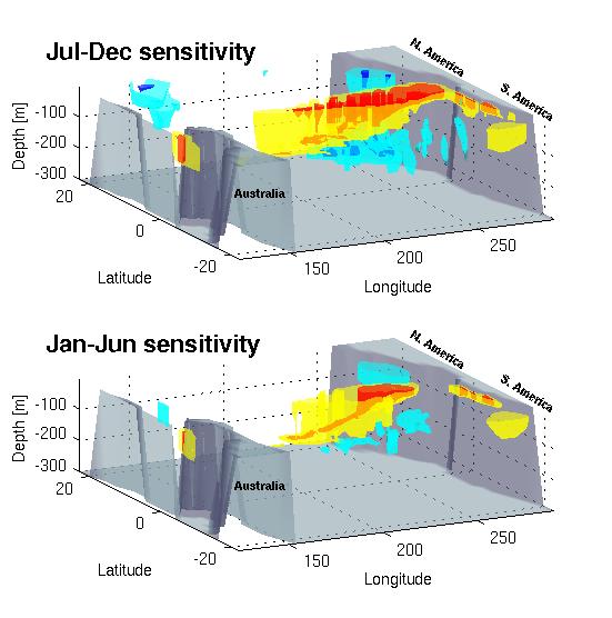
Sensitivity of East Pacific basic stratification to temperature in the equatorial Pacific (thanks to Eli Galanti...)

Transfer functions:

Climate models are often tested against observations by comparing some global metric such as global surface temperature time series (in the context of global warming), or East Pacific sea surface temperature (NINO3 index, in the context of ENSO simulation and prediction). It is possible, unfortunately, that a model would simulate such global measures seemingly correctly although individual processes responsible for this metric are flawed in the model, yet their corresponding errors compensate, leading to a good fit of the global metric to observations. It is important, therefore, to test individual processes in these models in addition to such global metrics. An "individual processes" in this context involves an input and an output with a corresponding mathematical relation between them. An example of an individual process is the reflection of westward propagating Rossby waves in the tropical West Pacific (the input) into eastward propagating Kelvin waves (the output), as part of the El Nino cycle mechanism. Another example is the effect of sub-surface east Pacific ocean temperature (the input) on the sea surface temperature (the output). We introduced the methodology of "transfer functions", borrowed from the field of control engineering, to the testing of ocean and climate models. This is done by comparing individual processes between models and observations, when available. Even when no sufficient observations are available, it is possible to compare individual processes in different models, where inconsistencies between the models indicate that at least some of them are wrong (model consistency, of course, does not imply no errors...). Some examples of this line of work are given in the following papers [1, 2, 3, 4, 5]

Back to main research page